Conditional Formatting
Highlight Specific Cells below a given number
Highlight Specific Cells below a certain number
File example highlight specific numbers
Imagine you have a Stock List that when the number reaches a certain level it is time to reorder. There are many options you can use and Conditional Formatting is one them.
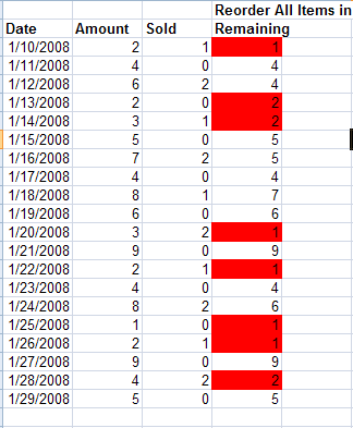
In this example we have four columns Date, Amount, Sold and Remaining.
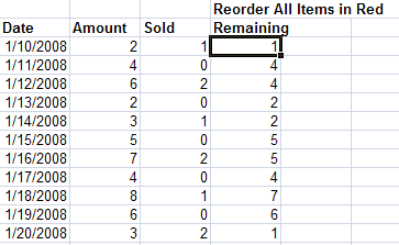
We want the Remaining column to show cells as red when they reach a certain level.
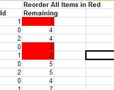
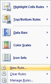
The simplest way to do this is to highlight the cells you want to show as red when they reach 2 or below. On the Home Ribbon click on Conditional Formatting

An optional menu will then open. Select the New Rule option and a dialog box will appear.
This will open the Conditional Formatting dialog box, click on Format only cells that contain and the Rule Description will now change.
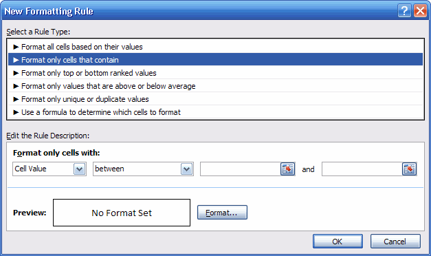
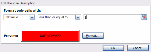
Use the Cell Value is option and select from the drop down list "less than or equal to" then the number you wish to order at, in our case it will be 2.
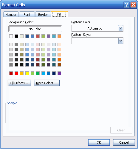
Select the Format button and change to the Fill tab. Select red and click on OK.
Your conditional formatting options should now be as shown below. Click on OK
Your table will now show all the items that you need to reorder.
Highlight cells using a list.
File example Conditional Formatting using a list
This Conditional Format option will allow you to use a list to highlight cells in your workbook. You can use this type of format to show below or above average scores using exact amounts, show items that reach a specific number for inventory purposes or show dates that are needed to be acted upon.
Create your table similar to the one below.
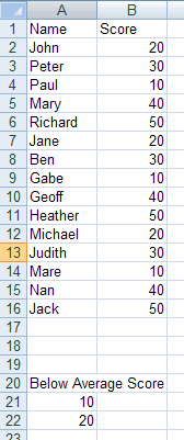
Highlight the column that has the score listed and go to Format > Conditional Formatting

This will open the Conditional Formatting dialog box, click on "Use a formula to determine which cells to format" the Rule Description will now change.
In the Edit the Rule Description box type in =countif then select cells A21 to A22 insert a , and then type in B2. Your formula should look like the one below.
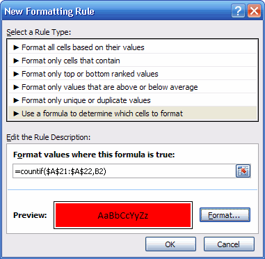
Select the Format button and change to the Fills tab. Select red then click on Ok.
Click on OK in the Conditional Formatting dialog box and your table should now look like this.
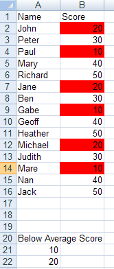
You can change the values below the Average Score to show different ranges. Please note that the Score and the Below Average Score must be the same.
If you would like help on this function please send me an email with a description of your problem and the version of excel you are using.