For this example of a Vlookup we will be using Teachers grading students.
Name your first Sheet Students by double clicking on Sheet1, when it is selected as shown below typ in students and press enter
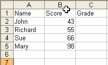
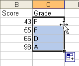
Create you sheet similar to the one shown below.
Double click on the Sheet2 tab and rename that Grades.
Fill out the Grades sheet as shown below.

Click on the Students tab.
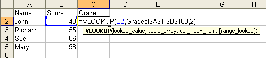
Move to cell C2. This is where we will insert the Vlookup. IMPORTANT! The table you are using for your vlookup, in this case the Grades must be sorted low to high and cannot contain doubles ie, you can't hav two 51's or if you are using text two people with the same name.
Your Vlookup function has several parts, Lookup_value which is the cell you want to use to get your grade from, in the Student table it is the Score column, the table_array is where you will be getting the grading information based on the students score. The col_index_num is where you will get the grade from, in this case the grade is in column 2 (the score is in column1).
Type in =vlookup(b2,Grades!$A$1:$B$100,2)
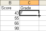
Press the enter key and your grade will now show in the cell. You will notice that there are Dollar ($) signs next some of the cell references, this is to make sure that they do not move when you copy the formula. To copy the formula down the row click on C2. You will notice a small black square on the bottom right of the cell, move the mouse over that square and it will turn into a + sign, double click on that and it will automatically fill the remaing cells down.
 |
 |
You can use the vlookup in a lot of situations to make your spreadsheet less work intensive.
If you have any questions please contact Richard and we will try to help you work out any problems you may have with your Vlookup's.