Compare Two Columns of Numbers
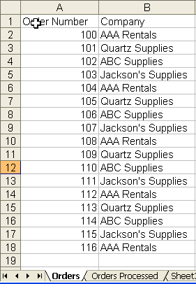
Create a simple spreadsheet similar to the one below or use an existing copy of one of your sheets.
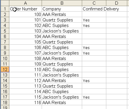
Orders sheet
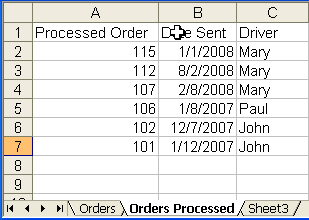
Orders Processed Sheet
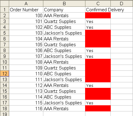
We now want to show on the first sheet what outstanding orders we have. Create a new heading on the Orders sheet called Confirmed Delivery.
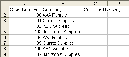
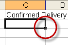
In C2 use the following formula
=IF(COUNTIF('Orders Processed'!$A$2:$A$20,A2)>0,"Yes","")
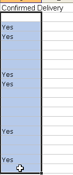
This formula will count the occurrences of the Order Number from the Orders Sheet in the Orders Processed sheet and if it finds a match will show Yes or if no match the cell will be empty. When you have entered the formula move back to that cell and you will see a small square on the bottom right of the cell . Double click on that square and it will automatically fill down the rest of the column.
This formula can be used in a variety of ways and makes it simpler to visually see any outstanding situations.
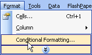
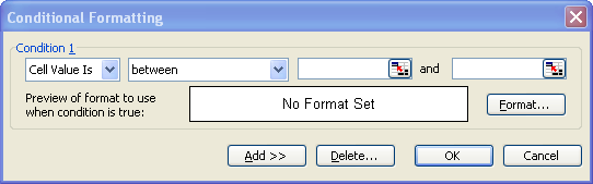
Another option you have is to highlight the outstanding Orders using conditional formatting. Follow the steps below to shade the cells that have outstanding orders in red.
Select the Confirmed Delivery column C2 to C18
Go to the Format Menu > Conditional Formatting
In the Conditional Formatting tab select Cell Value Is not equal to and type in Yes
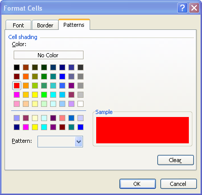
Click on the Format button and in the Patterns Tab select a color for the highlight, in this case I have selected Red, click on Ok.
Your Conditional Formatting should now look like this.
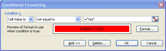
Click on Ok and your empty cells will now show red shading.